Now that confidentiality constraints have expired, I can share details about two sports-tracking systems I built in the early 2000s. To my knowledge, these were among the earliest of their kind: real-time multi-camera tracking on outdoor race circuits, streaming state vectors (not video) to remote clients, running on commodity x86 CPUs:
- Speedway (2003): tracking four motorcycles around a stadium dirt oval.
- Greyhound (2004-2005): tracking six dogs and a mechanical hare at a racetrack.
Both ran live, streamed data to dial-up clients, and had to work on hardware that a modern doorbell camera would trivially outperform. That scarcity shaped practices I still rely on. The project pages have the full details (the Greyhound write-up has more photos), but here’s a summary of what shipped and what I learned.
What shipped under tight constraints
When these systems went live, OpenCV was a fledgling v0.x, AlexNet was years away, and a Pentium 4 delivered roughly 12 GFLOPS – about 0.012 TOPS in modern terms. No practical GPGPU. 1 GB of RAM if you were lucky. Interlaced PAL video at 25 fps.
| System | Cameras | Compute | Objects | End‑to‑End Latency | Notable Tricks |
|---|---|---|---|---|---|
| Speedway | 9 × PAL CCTV | 3 × Pentium 4 | 4 motorcycles | <200 ms | SSE2 color kernels, helmet‑based identity hints |
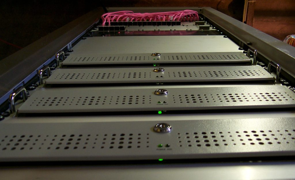
| Greyhound | 52 × PAL CCTV | 9 × Pentium 4 | 6 dogs + hare | <220 ms | 64×16 analog video matrix; 1‑D “track‑unwrapped” EKF |
The constraints dictated everything. Interlaced PAL meant I processed single fields only – half the vertical resolution meant half the processing load. No GPU meant hand-rolled SIMD, lookup-table colour classifiers, and aggressive early-exit logic. Dial-up users meant I couldn’t stream video; instead I sent state vectors under 1 kB per frame and let client-side software render a 3D view. Dust, rain, and floodlight glare meant per-pixel variance masks and automatic camera failover when things went wrong (which they did, regularly).
The geometry-first approach was the key insight. Both tracks were ovals, so I “unwrapped” them to a 1-D arc-length coordinate. Each camera produced noisy observations along that arc; a single extended Kalman filter fused them into smooth trajectories. Occlusions became gaps in 1-D space rather than hard re-identification problems in 2-D. Simple gating with Mahalanobis distance outperformed fancier global solvers – partly because it was fast, partly because the fancier solvers didn’t exist yet in any form I could run.
I also learned to design for failure early. Camera-by-camera health scores let the filter automatically de-weight dodgy inputs. Fixed time budgets per pipeline stage, with watchdogs that shrank ROIs or shortened association windows when compute spiked. The goal was graceful degradation: better to track three dogs confidently than six dogs badly.
One thing I got wrong initially: I underestimated how much the mechanical hare would confuse the system. It moved differently from the dogs – faster acceleration, no gait pattern – and my early motion priors kept trying to treat it as an outlier. I ended up giving it its own model with separate dynamics, which in retrospect was obvious.
What still applies
I’ve built a lot of systems since then, and the lessons from 2003-2005 keep showing up.
Geometry still wins. Deep learning has changed what’s possible, but homographies, EKFs, and motion priors still reduce how much your models have to learn. Smaller models, fewer labels, faster inference.
Bandwidth-first design still matters. On-device inference with lightweight telemetry uplinks (not video) lowers cost, improves privacy, and survives bad connectivity. The dial-up constraint turned out to be good training for cellular IoT.
Designing for failure is still underrated. Self-healing nodes, health telemetry, and graceful degradation matter as much as your model’s mAP. Maybe more, because mAP is measured in the lab and failures happen in the field.
Scarcity clarifies thinking. Whether you’re squeezing hand-rolled kernels onto a Pentium 4 or quantising a detector onto a 3-5 W edge accelerator, limited compute forces you to really understand your problem. I’ve seen teams with unlimited cloud budget build worse systems than teams with a $50 hardware target, because the $50 constraint made them think harder about what actually mattered.
Twenty years later, the hardware fits in a matchbox and the models are unrecognisably better. But the hard part was never just the compute. It was knowing what to spend it on.

